AI for Comedy

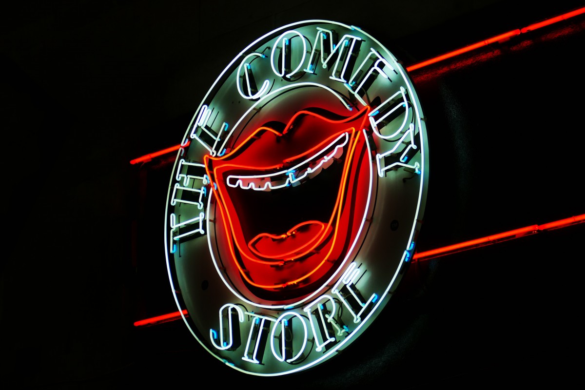
Which celebrity do you resemble? We sat down with our amusing partners at the Boom Chicago comedy theater in Amsterdam for a brainstorm session to see what Data Science could do for their shows. Someone remarked that it would be cool to use machine learning to build a celebrity lookalike matching system for visitors of the show. So we built an app.

In our app, we use Machine Learning to calculate the distance between a visitor’s face and a set of celebrity faces to find a lookalike, using the latest research in facial recognition. We then morph their face into that of their celebrity match using the latest research in Generative Adversarial Networks: the StyleGAN.

This current article dives into the most important background of our new application: generative networks. It is both written as a showcase of what current generative algorithms in deep learning can do and imply for the future, and a way to learn more about them by writing about how they work. I will save you from mathematical formulas and hope to provide you with an intuitive understanding of generative networks and our use of this type of algorithm. Note that you do have to have some basic knowledge of how (convolutional) neural networks work.

I’ll start with some fun historical context. Then I’ll explain autoencoders and generative networks, both architectures that can be used to generate (face) images. After that, I’ll go deeper into explaining the functioning behind the StyleGAN, which is the star of our application. When we have settled the necessary background, I’ll go into the specifics of what we’ve built, and close off with the big picture of what generative networks could do for us in the future.

People Who Do Not Exist

Image credit

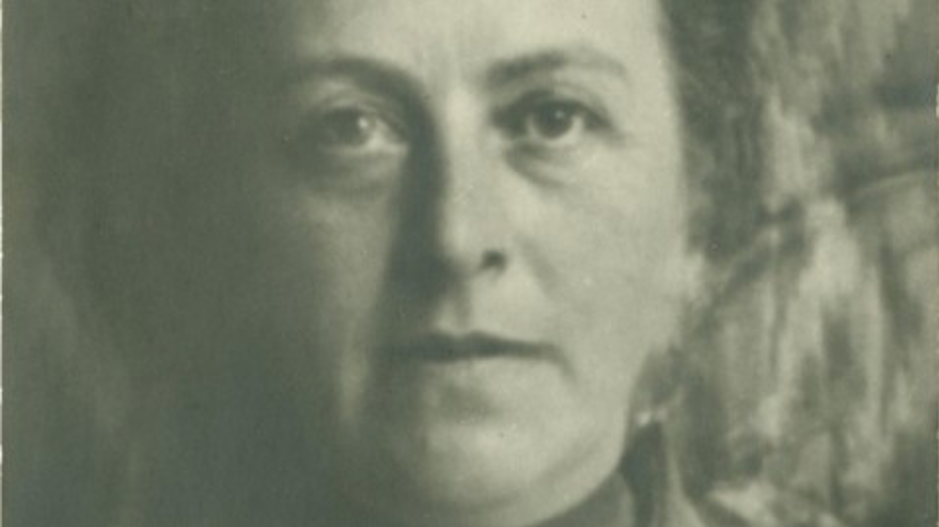
The uncanny lady in the above picture does not exist, and never has. So, what or whom is this a picture of — who is she? She is a composite photograph, that being the blending of two or more images into one, created by the philosopher Ludwig Wittgenstein. It is quite literally a family portrait, of himself and his three sisters.

Wittgenstein was interested in composite photography because to him this could bring to light the commonalities between members of a category, in this case “face”, or perhaps “family”. Such investigations may have marked the start of the development of his theory of Family Resemblance, where he postulated that neither necessary nor sufficient features can be identified for membership of any given category, but where a category represents instead a continuous overlap between its members, analogous to how no individual thread in a rope extends its distance.

This is true for any category, except for strictly mathematical objects, such as “square”, and those for which we’ve set conscious boundaries, such as the legal drinking age. Chairs, for a canonical example, prototypically have a seat, legs, and a back to lean against. Yet, one can easily dream up examples that jeopardise such strict definition. Bean-bag chairs may be sat on but lack the legs and back, and artistic instances may well do away with this whole sitting business entirely. Likewise, there isn’t a strict definition to be found for what a face really is and is best conceived as an interwoven set of features that all contribute in their own way. Of course, to us Data Scientists, this is no surprising find at all, as this is exactly what we would expect from training a classifier!

The creation of these compositions used to involve a rather laborious practice, where subjects had to sit still in the same exact position, using repeated limited exposure, so that big brother Ludwig had to torture his poor sisterhood using head-holders such as those depicted below, in which they must have sat patiently for quite some time as the photographic plate absorbed the light. No easy feat, but they came from a very strict household.

Later on, one could do this a bit easier using computers, where now we can easily overlay digital images to facilitate a similar blend. In fact, it’s something we’ve made use of in our app. This does however still require a strict match in angle between the two pictures. The ears should cover the ears, the eyes the eyes, mouth on mouth, and so on, just as in the example of the Wittgensteins. At present, modern machine learning techniques allow us to create similar such blends much more dynamically, with many fewer restrictions. Using generative algorithms, we can now not only generate images of people who do not exist , as Wittgenstein has, but we can also generate images of people who do exist; and we may then transform these images in various ways to our liking. Have you ever wondered what you’d look like with long hair, glasses and a mustache? Me neither, but we may now investigate these matters anyway.

Deep Learning and Generative Algorithms

Just as machine learning, and deep learning in particular, has taken over many other aspects of computer vision, so it has this niche of creating images of people that do not exist — and in extension, people who do exist, and the above mentioned facial transformations. Note that while we focus on (images of) faces in this article, as has much of the supporting literature, generative algorithms can in principle learn to generate anything at all, as long as you have a large amount of training data. You can also generate bedrooms , poetry, fireworks , and so on, given that you provide it enough data representative of the category.

There are essentially two ways by which you can generate images using deep learning: through generative adversarial networks, and through variational autoencoders. In our app, we made use of the StyleGAN, which is an instance of a generative adversarial network, an architecture that is markedly different from autoencoders. However, I will explain the autoencoders first, as they provide a great window on what the concept of a latent space is, which is such a crucial element in all of the generative architectures.

Autoencoders

Autoencoders are a neural network architecture of the unsupervised variety. That is, they are quite unlike a regular classifier, where you provide your dataset with labels and let the network discern between those. What autoencoders do is learn to reconstruct their input using fewer parameters, whereby the input serves as its own label. For images this means that you take an input picture, which is mathematically nothing more than a vector of its pixel values, and train a network to reconstruct facsimile output, taking as its loss function the pixel-to-pixel distance between the input and output. This is also called reconstruction loss, as reconstruction is the main objective of an autoencoder.

The nifty trick here is that the hidden layers in the network have fewer dimensions than the image that it takes in, thus causing the network to encode that image into a lower dimension by force of sheer economy: the layers in your network cannot just store the values of all the pixels — which you provide as input — but must instead learn a condensed representation of those pixels, such that it can recreate that image from that condensed representation. This condensed representation is what we call a latent space, typically denoted by Z. You can get Z by taking the output of the bottleneck, which is the sparsest hidden layer in the middle of the network. A latent space is called ‘latent’ because it is hidden, and ‘space’ because it is a compressed subspace of our original input space.

Now if you train the network on a large number of face images, such that it can reliably reproduce its input image, you could then take its latent space and consider what is to the left of it the encoder, and what is to the right of it the decoder. The business of the encoder is to translate the image into the latent space, and the business of the decoder is to generate from that latent space the image that the latent space is supposed to represent.

Because our latent subspace can no longer contain the pixel information of the original image (it isn’t allowed enough space), it has to get clever and store more general information about that image. For example, instead of encoding a blue square in terms of the amount of blue pixels it contains, you could instead describe that square using many fewer paramaters, such as the shape, the size, and the color, or rather the features of the square. The encoder does likewise for faces, encoding them into features, ranging from the general shape of the face to the nose down to the way your hair flows.

Variational Autoencoders

Autoencoders can be useful in, among other things, compression. You could for example have an encoder and a decoder on different devices, allowing you to send much smaller packages between your devices. Traditional autoencoders lack the ability however to generate new data, because although the latent space can inform the reconstruction of a particular image, changing it in any way, or presenting it with a new vector, will likely result in some kind of modern art, because its latent space is discontinuous.

The above pictures is an example of a discontinous latent space. The different colors correspond to the different digits of the famous MNIST dataset. As you can see, the areas in the latent space corresponding to certain samples are clustered away from each other. If you were to sample from this space in the area where the ? is drawn, then you get nothing in the output, because the decoder hasn’t learned how to deal with that region. It however makes sense that the encoder makes these distinct clusters, as it poses an easier question to the decoder: there is little confusion as to ‘what is where’. This is good for replication, but not generation, because you can’t sample from those regions, and you basically have no idea where the regions that do contain information are in the space, as the network can put anything anywhere it likes.

Variational autoencoders solve this problem by forcing the network to encode a latent space that is continuous by design. This is done in two ways, first by forcing local continuity, and second by forcing global continuity. The local continuity is forced as follows: instead of mapping its input to a latent space of size n, it instead outputs two vectors of size n: a vector of means, μ, and a vector of standard deviations, σ. The network then randomly samples its latent space from those two vectors, with each random variable corresponding to the ith mean and standard deviation from those two vectors. The reason for this is that if you take the mean and standard deviation of your inputs, and then sample from this probability distribution, you get the area around a point rather than just a single point. Now you’re teaching the decoder to deal with a continuity of points rather than leave local gaps in your feature encodings. Instead of decoding single points it now learns to decode distributions with slight variation.

Now that we’ve forced local continuity, we’re already better equipped to sample from our latent space, but we’re still left with some gaping holes between our features. Just as our traditional autoencoders encode features away from each other, a variational autoencoder can do the same thing, as it can learn very different means and standard deviations for each class, again giving the decoder an easier time in reconstruction. But this is still bad for generation.

It turns out there is a way to drive these features together, which is by giving the network an award if it drives the features together. The traditional autoencoder is awarded for a good reconstruction, but the variational autoencoder is now also awarded for encoding a latent space that is normally distributed. The way this is done is by adding a Kullback-Leibler divergence to the loss function. What this does is measure how much two probability distributions diverge from each other. In the case of variational autoencoders, this measures the divergence between the distribution of the latent space and a multi-dimensional normal distribution. This is, in the case of VAEs, minimised when the mean is 0 and the standard deviation is 1. If we only optimised for KL loss, then what we would end up with is a distribution around the center that encodes no meaning whatsoever, as everything has to maximally scatter, and any structure in this space is punished by the KL loss.

However, we can play a back and forth between the reconstruction loss and the KL divergence together and get just what we want. The reconstruction objective drives to encode features into clearly distinct regions, maximising the information to the decoder, but the KL divergence punishes this tendency to drive them apart and gathers everything round its center. Together they encode features into distinct, locally continuous regions, that nevertheless hug together closely, achieving global continuity.

Entanglement

Another advantage of adding KL divergence to the objective function, is to factor out feature entanglement. Feature entanglement happens when the encoder encodes features into multiple dimensions because it just doesn’t care. This means that if we want to change just the nose of our face image, we would end up also changing the ears, or mouth, or something else. Or some other parts of the nose would be elsewhere in the latent space. Disentangling a latent space means that we have dimensions that correspond to no more than one feature. Since the KL divergence drives the latent space closely around its mean of 0 and standard deviation of 1, the network is punished if it encodes information in a new dimension. But since spreading information around, fulfilling the wishes of the KL divergence, allows no information content at all, the network is therefore incentivised to do this anyway but be economical about it. No messing around with a dimension here and a dimension there. A major improvement in VAE quality was found in the beta-VAE, which does nothing more than making the network care even more about the KL divergence in the loss function.

It’s important to keep in mind the notion of a latent space, or feature space, and its issues with entanglement as we go on to the second way of generating (images): GANs, short for Generative Adversarial Networks. GANs have been producing a lot of impressive results recently, and get most of the attention in generating-stuff-land, but recent work on VAEs has shown that they are no slouch either.

Generative Adversarial Networks

In 2014, the AI-researcher Ian Goodfellow came up with Generative Adversarial Networks (GANs) in an inebriated tour de force. Legend has it that after he stumbled upon the idea while chatting with friends in a bar, he took an Irish exit home to code up an example, which to his surprise and to our continuous delight, actually worked, and subsequently spawned an entirely new field of research around deep learning.

The reasoning goes as follows: just as you can make a classifier learn the difference between cats and dogs, you can make a classifier that distinguishes between pictures that are real and pictures that are generated.As adversarial already implies, (two) networks are set up against each other. One network, the generator, attempts to replicate from a distribution of real images that it is trained on, and the discriminator then has to figure out whether this is a real or a fake: an image from the dataset, or an image generated by the generator.

The goal of the generator is to fool the discriminator, and the goal of the discriminator is to spot the fake. A good analogy is that of an art forger, such as the case of Wolfgang Beltracchi. Beltracchi is an interesting example because he doesn’t directly copy paintings, but rather fills imaginary holes in their repertoires. This is a good analogy to what a GAN does, because it should generate new faces, and not just replicate its training data. If we wanted mere replication, we’d have stuck with our faithful regular autoencoders.

As the art forger improves on making paintings that look ever more like the artists they’re copying, or mimicking, the discriminator must improve its discernment. At first the fakes may be easily identifiable, because, for example, the paint leaves obvious clues that it has recently dried. But the forger will soon figure this out, and improve the quality of his painting, at which point the discriminator must find out better modes of rejection. In this cat and mouse game both networks improve at their job, to the point where neither can improve any more: the point where the generated image is so good that the discriminator can no longer discern between the original and the fake, and the generator can no longer change anything about what it generates to improve its score. This point, where neither ‘player’ can improve their game, is called a Nash equilibrium.

More formally, the way GANs work is that the generator network starts with some noise vector Z, which is the GAN’s latent space, and passes it through the generator network to get an output. The discriminator network then must decide whether this concoction is either part of the original distribution (real) or created by the generator (fake). The networks are trained together playing what is called a Minimax game.

The discriminator is trying to always be correct in its assessment, by maximizing the amount of times it labels real data as ‘real’, and generated data as ‘fake’. The generator is trying to produce good images, by minimizing the amount of times the generated data is labeled as ‘fake’, or conversely, maximizing the amount of times the discriminator is fooled. It is important to train the generator along with the discriminator in gradual steps, playing them up against each other, to avoid one being blatantly better never allowing the other any useful feedback.

We find a Nash equilibrium exactly where neither the generator nor the discriminator can make any improvements on their objectives. However, what happens in practice is that the GAN gets stuck in a local optimum, or a local Nash equilibrium, where the two networks oscillate on what is not a good image at all, which can lead to some weird results that don’t make much sense at all. (Some that people have put forward as art and sold for almost half a million dollars. Not a bad outcome of a shitty GAN.)

We have two main goals with GANs in the context of generating face images. The first is to generate images of high quality, which on the one hand means producing a legitimate forgery a la Beltracchi, but also one of high resolution; and the other goal is to produce disentangled latent spaces. All this without too much hassle. With respect to these goals, we have two big problems with the original GAN architecture. Firstly, the original GAN produces images of rather low quality. And secondly, the original latent vector Z is still latent spaghetti, such that we have no control over its output.

Fortunately, a lot has been improved on the GAN architecture since Goodfellow’s initial code and paper from 2014. I won’t go over all these innovations but will get into some big improvements that distinguish the original GANs from the star of the show in our application: the StyleGAN.

Progressively Growing Images

The StyleGAN innovates on one of its more immediate predecessors, namely the Progressive GAN, or ProGAN for short. It’s difficult to generate images of high quality, because the generator must learn to generate both large structure and fine details at the same time. Training is unstable and slow because generating larger images involves a much longer and more complicated process (there are many more pixels to change).

Various solutions to these (and many other) problems have been explored. One successful solution is the Wasserstein GAN, which improves the GAN by computing a different objective function very similar to what the VAEs do: force the latent space in a certain distribution. Read more about this here.

The ProGAN and the StyleGAN build on the success of the Wasserstein GAN, but don’t make further changes to the objective function. The primary contribution of the ProGAN is a training methodology where the network starts with a small image, progressively increasing its resolution by adding (convolutional) layers to the network. It starts with a low (4×4) resolution, doubling onward to its ultimate output (1024×1024). This progressive up-sampling is what allows a high-resolution output because the network learns base features first and gradually increases details on the image, thus not having to do it all at once. As shown below. The generator is grown as a mirror image of the discriminator, so at no point will one overpower the other.

The power of the ProGAN lies in how it deals with features of various levels. Base features can be understood as the rough shape of the face that is depicted, and the pose that it is in. As the resolution increases, more room for detail emerges for detailed, fine features, such as the shape of the nose, the color of the hair, and so on. Because the ProGAN increases the resolution gradually, it is at each step asking a much ‘simpler question’ of the network, which improves the stability and increases speed.

The StyleGAN

The ProGAN already creates realistic-looking faces, but they’re missing some of the finer details. More importantly, we still have an entangled latent space. The StyleGAN also progressively grows its images but addresses these problems by first disentangling the latent space and then then using that improved latent space to inform the growing of the image step-by-step.

Mapping network

One important improvement is the mapping network. The mapping network is part of the generator, and it is composed of a bunch of fully connected layers. It is there to turn our noise vector Z into W, before it moves on through the rest of the network. Compare the two architectures below, comparing the ProGAN to the newer architecture of the StyleGAN.

Why use the mapping network to go to W first? To reduce entanglement. Going from Z to W allows the generator to turn Z into any kind of distribution that it likes, because it isn’t forced to encode it in any predetermined region. This way it does not have to encode any bias that exists in the training set. For example, our dataset may be lacking men with long hair. So, at this point in our data distribution, we have a gap. Without W, we would now have a warped latent space, as the network learns that men apparently don’t have long hair. Going from Z to W allows you to ‘unwarp’ space such that it can still allow generating men with long hair, even when they are absent from the dataset. This reduces entangling because, in this case, ‘masculinity’ is no longer strongly associated with ‘short hair’. The authors postulate that the reason that the mapping network does all these nice things, is because it is more economic to generate high quality output from disentangled vectors than entangled ones.

Style Modules

A second important improvement is style modules. The StyleGAN lends its name from the Style-transfer literature, which you may know from these kinds of images, where objects are transformed into their counterparts of famous artists, controlling the finer details of the image. Forcing them in the “style” of the painter but keeping the larger structure.

The way the StyleGAN controls the details of the generated image is by plugging in the disentangled W at every level of the generation process through blending layers called AdaIN. For each resolution, W blends in twice, hence its dimension of (512,18), where for the nine resolutions, there are two dimensions for each. For how the AdaIN works mathematically, I’d refer you to the paper, but suffice to say it affects the features of that resolution of the image generation process one level at a time. The levels are distinguished as follows: coarse, up to 8×8, affects general pose, hair style: the base features; middle, resolution of 16×16 to 32×32, affects finer facial features, eyes open/closed, etc; and fine, resolution of 64×64+, affects colors and fine features. Before each blending, noise is also added, to control what they call ‘stochastic features’, such as freckles, small marks, and the exact way hair is flowing. This way we build up the image like the ProGAN, but we control features at multiple resolutions by blending in our disentangled W step-by-step, rather than just at the beginning.

At the beginning of the synthesis network, there is a learned constant. This is the seed of the network, where ‘normally’ Z would go through. This seed is then optimized during the training process, because it is part of backpropagation. It is not explained why this helps in the paper, but it works presumably because it leaves all the control up to the disentangled W.

Thankfully, we can download the fully trained network from Nvidia, saving us countless hours of expensive training using the best TPU/GPUs on a massive dataset, which in their case is the Flickr faces dataset, consisting of 70k high-quality face images.

From Face to Space

Now that we’ve established how we can use the StyleGAN to generate faces using disentangled latent vectors, we can get to the next step of our celebrity matching algorithm. What we want to do now, is take an image of our own choosing and generate a latent vector from that image, such that we can play around with it, by changing parts, or by blending it with other images. Luckily, some inventive enthusiasts have forked Nvidia’s StyleGAN code and improved it to provide just this functionality. One of these is a legendary figure who goes by the name Puzer. He figured that you could learn latent representations of input images using some nifty tricks.

Something (not very nifty) you could do, is to use an average latent vector resulting in an average face, with respect to your training data. You could then compute an L2 loss comparing your image of choice, and your generated image pixel by pixel. Assuming you align your images so that the ears cover the ears, the eyes the eyes, mouth the mouth, and so on, that could work. Additionally, you could use face masks, where only those pixels that are on the face count towards your loss. By freezing the weights of the generator network, you can iteratively update your latent vector only, minimizing your loss between images. In the end, when your loss is very small, you should end up with the latent vector that produces your target image, or kind of.

In practice however, this starts off in the right direction, but gets stuck in a local minimum. It’s probably comparing the images too specifically. It’s also slow. Puzer innovated on this basic idea with a better idea named the perceptual loss trick (very nifty), which computes the loss not between pixels of the image, but between its features. It works as follows: you take a network that is already trained on many images. You then process both your target image, and your generated image through this network, and take from both these networks one of the later layers, which typically encode the features found in an image. Then instead of computing a pixel-by-pixel loss you compute the difference between your target image and generated image in semantic space, which is like a latent space, and you generate it from the image rather than the reverse. (You can’t use it to generate images.) Specifically, Puzer took the 9th layer from VGG16, which is a network pre-trained on ImageNet, and computed a mean squared error between their outputs, asking the question: how different are the features in these images? Doing this works beautifully well, but it’s also slow.

What if you could be even niftier? Maybe by not starting with a random image, but by one that already looks a little bit like your target image. But how? That is what a man known by the name of Pbaylies figured out. He forked Puzer’s code, and made it not slow. What he did was generate a lot of images using some random latent code for each image. What he then had was a lot of images with a label: their latent code. He trained a ResNet, a network that works well with images, similar to VGG16, to go from image to latent code. Now that you have a starting point you only have to update the image from that starting point, requiring many fewer steps. From our experience, Pbaylies’s approach is about five times quicker than using Puzer’s stategy only. Very nifty indeed. He made some other improvements too, which you can look up in the repo.

A recent paper has come out where another approach is used that is very similar. Better and niftier ways of going from images to spaces will probably come forth soon, along with better GANs. As of now, what we have is a way to get a latent space from any image we want. Which opens up many possibilities of playing around with that latent space to produce fun results.

Moving Through Feature Space

We can move around our latent space, which is disentangled and continuous. For example, we can change some part of the input Z of a face output and see the output change in some way that still is a face.

Because we have a continuous, disentangled latent space, we can explore the space between two faces, and expect them to gradually morph into each other. This works because we can do basic vector arithmetic on our latent space. Which is the kind of effect we were going for and you’ve already seen by now. This is simply done by looping over two latent spaces, starting at one, and then gradually taking larger proportions of the other face, while taking smaller proportions of the starting face, resulting in a smooth transition. We can then also create children of two parents by taking equal proportions of their latent spaces. A kind of pre-Mendelian conception of genetics, where children are really a fair blend of their parents.

Changing Facial Features

Now one problem is that even though our meddling with the input will at least result in a face, we still don’t know where what is in the latent space: which parts of the latent space correspond to, say, someone’s beard? Fortunately, we don’t have to know or learn by tedious trial and error. Because of some additional nifty thinking by Puzer, we can also mess around with facial features, at levels middle and high. Middle levels in this case corresponding to the individual facial features such as hair and the senses, and high meaning composite features such as gender and age, affecting multiple features at once.

What Puzer did was generate a whole lot of faces using random latent vectors. He then classified them into groups: smiling / not smiling, young / old, male / female. Using his latent space as features, he trained a linear regression model to predict those labels. The weights of that linear model then represent the direction in feature space you need to go in to produce that output. You could also do this by taking existing face-classifiers on whatever feature you’re interested in changing.

In gradual steps, you can make a person laugh more, or less, by tuning those parts of the latent vector that are involved in this effect, such as the curvature of the mouth but also the wrinkles around the eyes. Because the facial features are disentangled, we can find linear directions in our latent space and go from man to woman, not smiling to smiling, young to old. In our app, we used the laughing direction already found by Puzer to make people laugh. Literally.

Interestingly, we find some entanglement in this laughing effect. It seems that the more you make someone smile, the more likely they are to get glasses too. It could be that Puzer took a lot of smiling people with glasses in his dataset, or it could have entangled for another reason.

Measuring Entanglement

Apart from looking at the output. How can we figure out whether our latent space is really disentangled or not? The authors of the StyleGAN paper propose two new metrics: perceptual path length and linear separability. Perceptual path length means that you take two random outputs of the network, and then interpolate between them, and measure the distance in their VGG outputs (exactly like the ones Puzer used to determine the distance), and check that there aren’t any big ‘jumps’, such as a nose suddenly getting really big — or glasses appearing and then disappearing. From our experiments — and of course the authors’ own analysis — we can see that this is mostly sound.

Linear separability means that we can classify the inputs into binary classes, such as male/female, and young/old. From our experiments we can see that this is sound as well, as otherwise we would not be able to move our faces in these directions using only a linear model.

Generating high-quality images using generative adversarial networks is not easy, for the reasons discussed above, as well as other issues that we haven’t touched on. But thanks to the smart researchers at Nvidia and elsewhere, we can generate very impressive images using the StyleGAN, and in the future we’re likely to see even better results from even niftier architectures, as at just five years old, the research is very much still in its infancy.